From Sampling the Forest to Sampling the Error
A Spatial Sampling Decision Framework for Trustworthy Forest Carbon-Stock Accounting
How should a limited verification budget be spent when every candidate plot competes to reduce uncertainty? On 576 fixed 20 m × 20 m LiDAR plots at Saihanba, we treat sampling as a decision problem in the error field rather than in the forest, and show that aligning plot placement with the error structure roughly doubles verification sample efficiency.
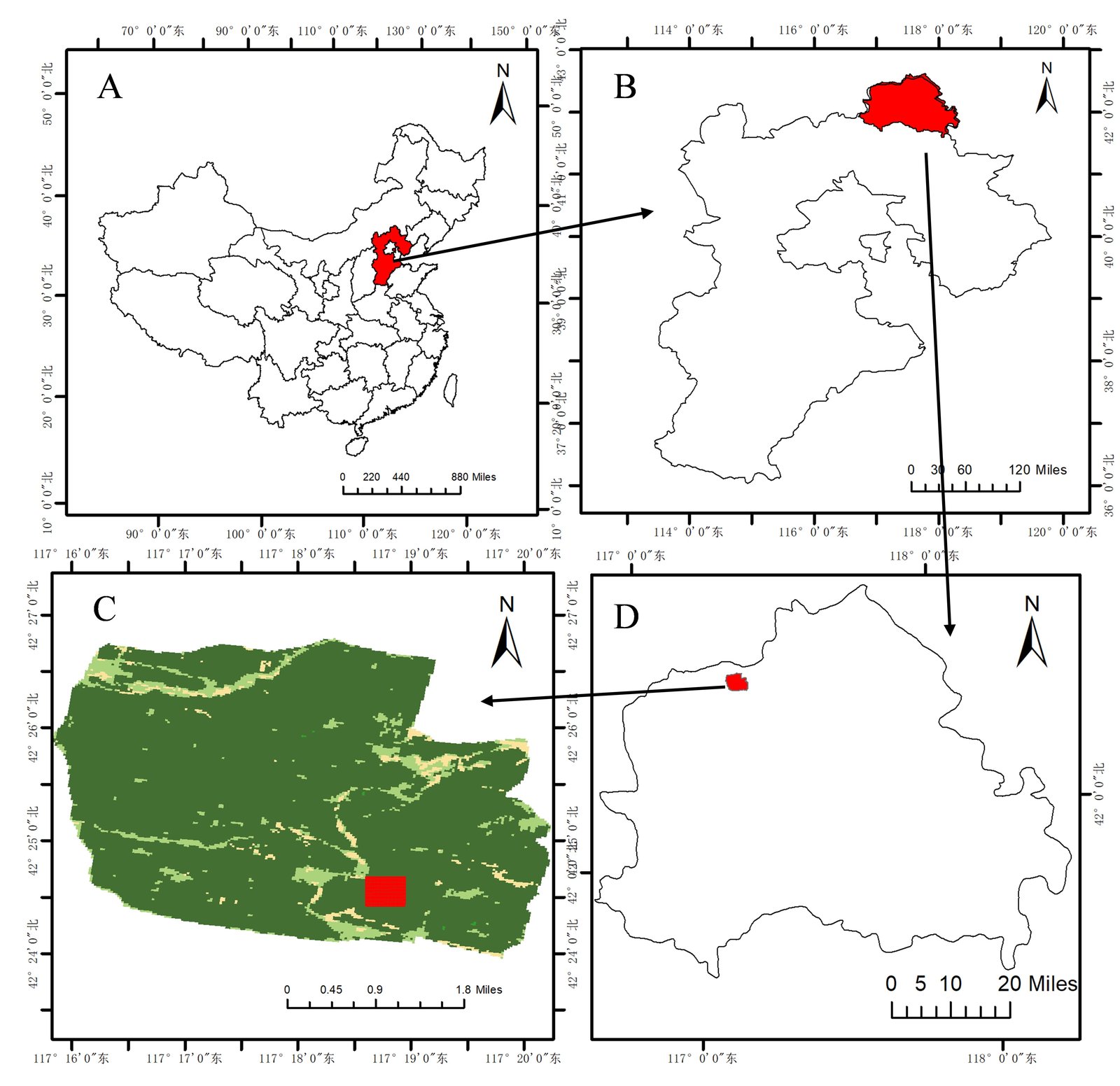
Figure 1 · Saihanba study area: (A) province-level location within China, (B) county-level location within the province, (C) plot location within the forest-farm remotely sensed imagery, (D) plot position within the county
Figure 2 · Tilted top-down view of individual tree crowns in the study area (2024, extruded by tree height, colored by per-tree carbon stock)
Study area, data, and the SMP-cLHS framework
576 fixed 20 m × 20 m LiDAR plots
Airborne LiDAR yields a canopy height model; individual tree crowns are segmented; single-tree carbon is estimated from crown geometry and summed to the pixel containing the crown apex (t C/ha = tree carbon in kg ÷ 40). Across the 576 plots in 2024, mean carbon density is 58.85 t C/ha (SD 17.74, CV 30.1%). LiDAR DBH was spot-checked against 101 field-measured trees: relative RMSE 6.5% (2024, 88 matched trees), below the 10% threshold of the CCER methodology.
SMP-cLHS: sampling in error space
Histogram matching aligns the sample's NDVI and NIRv distributions to the population's (conditioned Latin hypercube stratification); simulated annealing then disperses plots in space under zonal quotas. The sampling attributes are exactly the feature space of the downstream model — only satellite-observable indices may influence plot selection, never carbon or LiDAR structure.
Seven estimators spanning attribute → space → fusion
| No. | Method | Information used |
|---|---|---|
| E1 | Quadratic regression on NDVI + NIRv | Attribute only (spectral) |
| E2 | IDW interpolation (p = 2) | Space only |
| E3 | Ordinary kriging (de-mean, interpolate, add back) | Space only |
| E4 | E1 regression surface + kriged residual correction | Additive fusion |
| E5 | w·E1 + (1−w)·E2, w a global LOO weight | Weighted fusion |
| E6 | w·E1 + (1−w)·E3, w a global LOO weight | Weighted fusion |
| E7 | Per-pixel fusion of E1 and E3 weighted by error maps | Per-pixel weighted fusion |
Why this design: three propositions from Gaussian-process conditional inference
Effective sample size is capped by correlation
Spatial correlation caps the effective number of independent samples in full-coverage information at about |D|/(2πℓ²). At Saihanba the direct carbon field (range ≈ 200 m) yields Neff ≈ 0.8 despite 576 pixels, while the regression-residual field (range ≈ 1.7 m) is nearly white noise. This is why adding remote-sensing pixels cannot improve the regional mean, yet a few ground plots buy a disproportionate gain.
Fusion never hurts
Conditioned on the plots, fusing the regression prior with kriging of its residual reduces posterior variance by the information gain G(S) — a non-negative quantity. Remote sensing plus ground verification is never worse than remote sensing alone.
The value of a plot is its conditional covariance
Adding a candidate plot j reduces the regional-mean variance by a quantity set by j's conditional covariance with the regional mean. The SMP objective is an operational approximation of this principle in attribute space.
Ground-truth validation
LiDAR vs field measurement: the direct check required by CCER
101 field-measured trees (girth converted to DBH, GPS-recorded) were matched to LiDAR tree crowns by geometric overlap (IoU > 0.5); LiDAR-estimated DBH is compared against the field value.
Auxiliary: cross-validation of the DBH conversion formula itself (height + crown → DBH)
The following compares four candidate conversion formulas. It measures formula fit quality and is not the CCER Table 35 ground-validation evidence above.
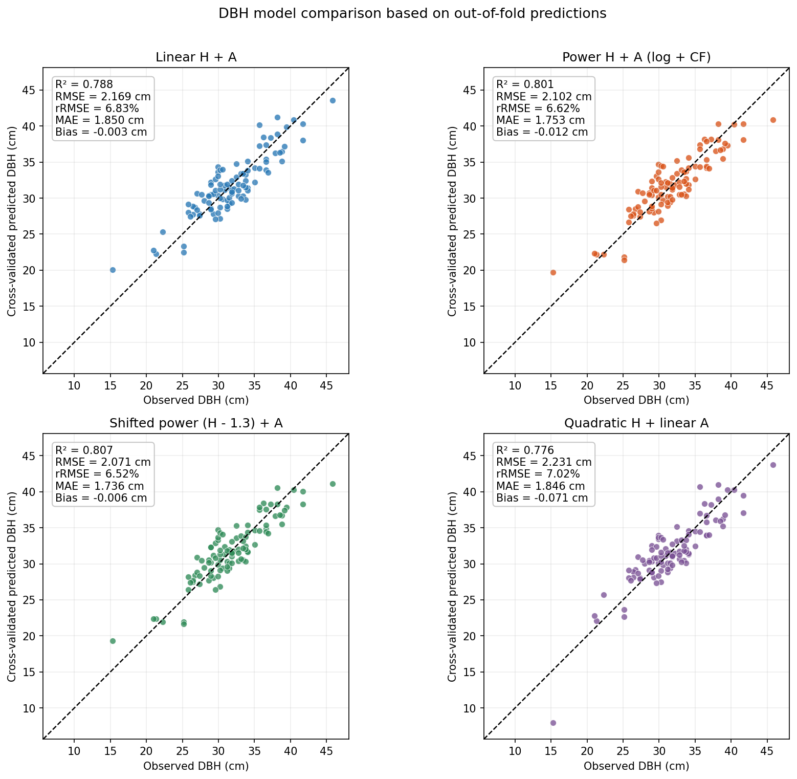
Figure 9 · DBH conversion: observed vs predicted (cross-validation)
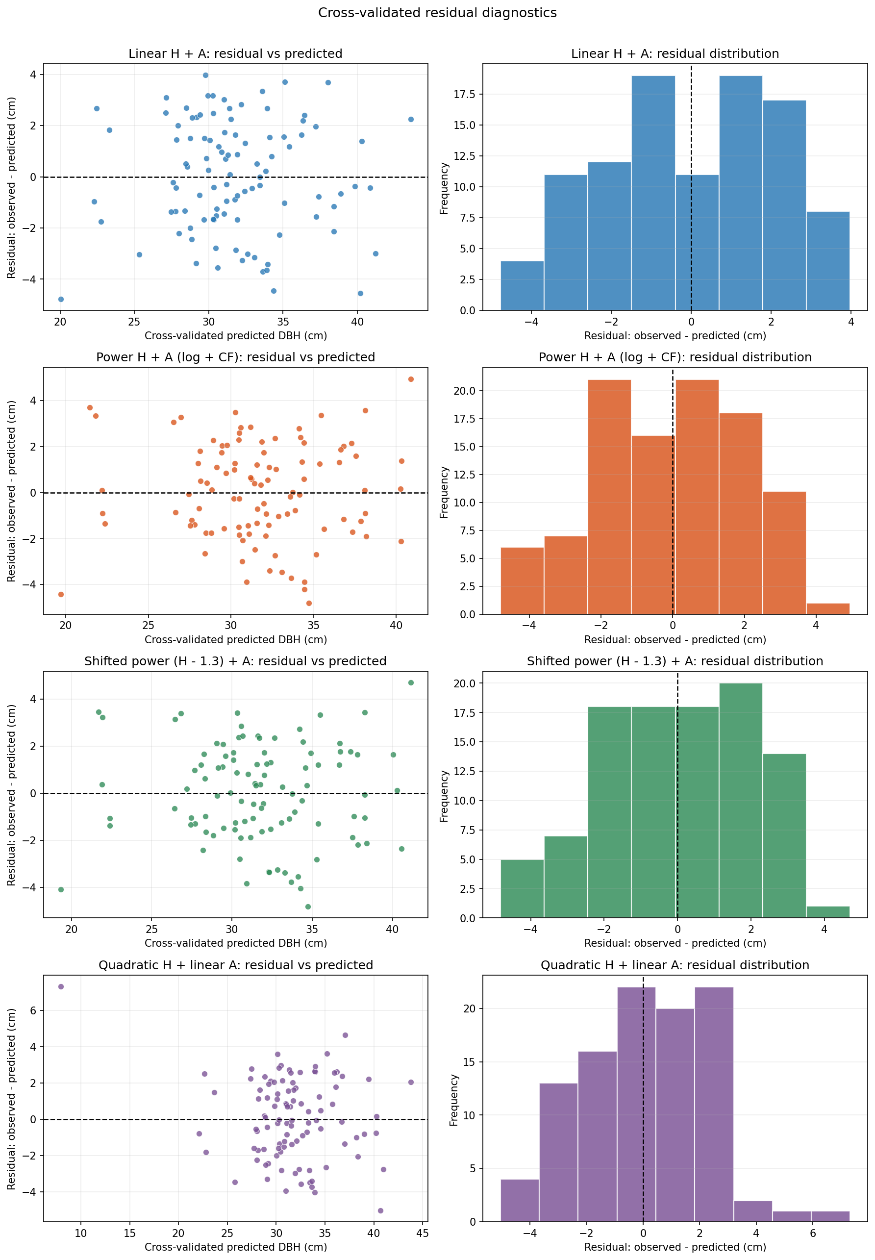
Figure 10 · DBH conversion: residual diagnostics
Limitations
(1) The evaluation truth is LiDAR-inverted, not field-measured
LiDAR single-tree DBH was validated against 101 measured trees (relative RMSE 6.5%), but the absolute accuracy of per-pixel stock still depends on the allometric equations, only 39.6% of the measured trees fall inside the study area, and the check stops at DBH as an intermediate variable.
(2) One study area, one date, one scale (~460 m square)
The NDVI distribution is strongly left-skewed (mean 0.82), and no perturbation analysis was run on the sensitivity of histogram matching to the low-NDVI tail. Scaling up requires recalibrating the variogram.
(3) LOO weights ignore error correlation
The leave-one-out weights of E5/E6 use inverse error variances and ignore the correlation between the two fused errors, which is in theory information the fusion could exploit.
(4) Simulated annealing is a stochastic search
Results across designs have converged over 20 seeds (small standard deviations), but a better layout search may still exist within the same objective.
(5) No independent prior-period observations
The design uses no independent prior-period observations. Should historical survey data independent of the 2024 inversion become available, the sampling attributes could be extended and the framework re-run end to end.